Categorical Modeling¶

The pygeostat.categorical module includes categorical modeling functions.

Hierarchical TPG Class¶

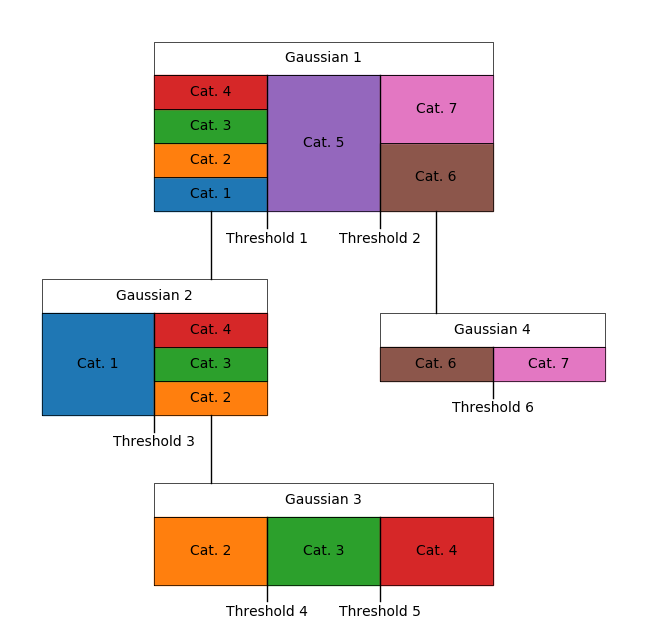
class pygeostat.categorical.HierTPG(mask, griddef=None, catdict=None)¶

Class for working with and executing the hierarchical truncated pluriGaussian simulation (HTPG) suite of programs. The object attributes permit minimal required arguments in each successive step, which is laid out in the example below

Parameters:

mask (dict) – dictionary that specifies the truncation mask. See the example below for the format, where the first level keys should proceed from ‘g1’,…,’g<ngauss>’. The second level keys should proceed from ‘t1’,…,’t<nthresh>’. The third level keys should always be ‘below’ and ‘above’. A dictionary is used for visual understanding of thresholds (t<x>) associated with each latent Gaussian variable (g<x>), and the categories above and below each threshold. The list/int values in the third dictionary level specify the category codes.
griddef (GridDef) – this is drawn from gsParams[‘data.griddef’] if None. An Error will return if griddef=None and gsParams[‘data.griddef’]=None.
catdict (dict) – optional dictionary that is formatted as {catcode : catname}, where the the catcodes should include all codes within mask.

Workflow Example:

import pygeostat as gs

# Define the mask.
mask = {'g1': {'t1': {'below': [1, 2, 3, 4], 'above': 5},
               't2': {'below': 5, 'above': [6, 7]}},
        'g2': {'t3': {'below': 1, 'above': [2, 3, 4]}},
        'g3': {'t4': {'below': 2, 'above': [3, 4]},
               't5': {'below': 3, 'above': 4}},
        'g4': {'t6': {'below': 6, 'above': 7}}}

# Define a grid-definition
griddef = gs.GridDef('120 5 10\n110 1205 10\n1 0.5 1.0')

# Initialize the HTPG object
htpg = gs.HierTPG(mask, griddef=griddef)

# Plot the mask to ensure that the appropriate dictionary mask was used
htpg.plot(figsize=(8, 8))

# Calculate the global and local thresholds, given declustered proportions
# and (optionally), a file that contains the local category proportions (trend)
htpg.thresholds(globprops, locpropfl=trend.flname, locthreshfl=outdir+'localthresh.gsb')

# Calculate the Gaussian variogram models that will truncate to the category
# proportions, given the categorical variograms
htpg.gaussvarg(vargs)

# Calculate the Gaussian variogram models that will truncate to the category
# proportions, given the categorical variograms
htpg.gaussvarg(vargs)

# Now that the truncation mask, Gaussian variogram models and locally varying
# thresholds are defined, the Gaussian data realizations may be imputed as
# the final step prior to simulation of the grid
htpg.cat2gauss(data, gaussdatadir, searchradii)

# After simulating the grids, the gauss2cat function may be used for truncating
# the Gaussian realizations, where the input Gaussian realization files (wild card)
# specifies the iterating realization number is input, along with the corresponding
# output file.
htpg.gauss2cat('gaussreal*.gsb', 'catreal*.gsb')

Code author: Ryan Barnett 2018-04-25

Plot¶

HierTPG.plot(cmap_cat=None, figsize=None)¶

Plot the truncation mask.

Parameters:	cmap_cat (dict) – dictionary formatted as {catcode: catcolor}. If None, drawn from gsParams[‘plotting.cmap_cat’] if its keys correspond with self.cats. figsize (tuple) – Figure size (width, height), which is the primary utility for ensuring that the bounding boxes of each category in the plot are appropriately dimensioned.

import pygeostat as gs
mask = {'g1': {'t1': {'below': [1, 2, 3, 4], 'above': 5},
               't2': {'below': 5, 'above': [6, 7]}},
        'g2': {'t3': {'below': 1, 'above': [2, 3, 4]}},
        'g3': {'t4': {'below': 2, 'above': [3, 4]},
               't5': {'below': 3, 'above': 4}},
        'g4': {'t6': {'below': 6, 'above': 7}}}

# Default grid definition
gs.gsParams['data.griddef'] = gs.GridDef('120 5 10\n110 1205 10\n1 0.5 1.0')

# Initialize the HTPG object
htpg = gs.HierTPG(mask)

# Plot the mask to ensure that the appropriate dictionary mask was used
htpg.plot(figsize=(8, 8))

Code author: Ryan Barnett 2018-04-25

Thresholds¶

HierTPG.thresholds(globprops, locpropfl=None, locthreshfl=None, exepath=None)¶

Execute the htpg_thresholds program, providing the global and (optionally) local thresholds.

Parameters:

globprops (list) – list of the declustered global category proportions, whose order should correspond with self.cats.
locpropfl (str) – optional file with local proportions. The file should align in dimensions with self.griddef. The columns in the file are assumed to be 1,…,ncat, and aligned with self.cats. Using this file activates the locally varying thresholds option.
locthreshfl (str) – locally varying thresholds are output to this file.
exepath (str) – path to the program ‘htpg_thresholds’, which defaults to the included pygeostat executable if None (only modify if using another compiled executable that is located in a different path)

Returns:

self.globthresh (list) – global thresholds
self.lothreshfl (str) – content may be loaded and plotted

Code author: Ryan Barnett 2018-04-25

Gaussian Variogram¶

HierTPG.gaussvarg(catvargs, plotcat=True, plotgauss=False, exepath=None)¶

Execute the htpg_gaussvarg program, providing Gaussian variograms to fit for input to imputation and simulation of the Gaussian latent variables.

Parameters:	catvargs (gs.Variogram ncat-list) – list of variogram objects that should have models initialized. The models should be fit to standardized indicator variograms for each category. If using locally varying thresholds, the variograms should be calculated on indicator residuals of the locally varying thresholds. catvargs – list of variogram objects that should have models initialized. should correspond with self.cats. plotgauss (bool) – plot the calculated Gaussian variograms. This defaults to False, since the experimental variograms (self.gaussvarg) must be fitted seperately (where they are presumably displayed). exepath (str) – path to the program ‘htpg_gaussvarg’, which defaults to the included pygeostat executable if None (only modify if using another compiled executable that is located in a different path)
Returns:	self.gaussvargs – A list of `gs.Variogram()` objects containing the experimental Gaussian variograms, which must be fit separately
Return type:	list

Code author: Ryan Barnett 2018-04-25

Cat 2 Gauss¶

HierTPG.cat2gauss(data, gaussdatadir, nreal=None, nprocess=None, nburnin=1, searchangs=(0.0, 0.0, 0.0), searchradii=(1e+21, 1e+21, 1e+21), searchn=24, exepath=None)¶

Execute the htpg_cat2gauss program, providing data realizations of the Gaussian latent variables.

Parameters:

data (DataFile) – data file, which must have its flname, x, y, z, and cat attributes initialized.
gaussdatadir (str) – directory where the Gaussian data realizations will be written to as ‘1.dat’,….,’<nreal>.dat’.
nreal (int) – number of data realizations to impute, which should be equal to the number of gridded realizations that will subsequently be generated. Drawn from gsParams[‘data.nreal’] if None.
nprocess (int) – the number of parallel processesing threads with which to execute the imputation. Drawn from gsParams[‘config.nprocess’] if None.
nburnin (int) – number of burn-in iterations for the Gibbs sequence, which should generally be between 1 (poorer results, but faster execution) and ~10 (better but slower execution).
searchangs (3-tuple) – angles of the search ellipsoid in the major, minor and vertical dirctions.
searchradii (3-tuple) – radii of the search ellipoid, which should generally be set to the maximum range of self.gaussvargs in the major, minor and vertical direction.
searchn (3-tuple) – the number of nearest neighbours to use for imputation. A rule of thumb is 24 for 2-D and 40 for 3-D, although less neighbours may be necessary for computational expense.
exepath (str) – path to the program ‘htpg_cat2gauss’, which defaults to the included pygeostat executable if None (only modify if using another compiled executable that is located in a different path)

Returns:

self.gaussdatafls (str nreal-list) (nreal files provide the Gaussian data realizations that) – may be input to simulation.
self.nreal (int) (number of imputed data realizations.)

Code author: Ryan Barnett 2018-04-25

Gauss 2 Cat¶

HierTPG.gauss2cat(simgaussfl, simcatfl, nprocess=None, exepath=None)¶

Execute the htpg_cat2gauss program, truncating simulated Gaussian variables into simulated categorical variables.

Parameters:	simgaussfl (str) – the file name with the simulated Gaussian values, where each Gaussian variable is assumed to be located in the 1,…,ngauss columns. The file name may include a wildcard ‘’, indicating that the realizations are located in dedicated files that are named by replacing the wildcard with 1,…,nreal. If using a wildcard in simgaussfl, a wildcard must be used in simcatfl. simcatfl* (str) – the file name with the output simulated categories. Refer to the description above for the optional wildcard. nprocess (int) – the number of parallel processesing threads with which to execute the truncation. Drawn from gsParams[‘config.nprocess’] if None. Only applied if a wildcard is used. exepath (str) – path to the program ‘htpg_gauss2cat’, which defaults to the included pygeostat executable if None (only modify if using another compiled executable that is located in a different path)
Returns:	self.gaussdatafls – nreal-list nreal files provide the categorical realizations.
Return type:	str

Code author: Ryan Barnett 2018-04-25

Calculate Proportions¶

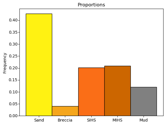
class pygeostat.categorical.Proportion(data, wt=False, catdict=None, cmap_cat=None)¶

Calculate/plot the weighted or unweighted categorical proportions of data and realizations.

Parameters:

data (DataFile) – must have its data.cat attribute initialized
wt (bool) – if True, the weighted proportion is calculated, but data.wts must be initialized
catdict (dict) – used for naming the category bins in the histogram; taken from data.catdict if initialized
cmap_cat (dict) – dictionary of category colors, formmated as {catcode: catcolor}, where the catcodes must align with the keys of self.catdict. If None, drawn from gsParams[‘plotting.cmap_cat’] if its keys align with self.catdict. Used on initialization to permit consistent coloring within plotting functions.

Returns:

self.props (pd.DataFrame) – category proportions
self.props_df (pd.DataFrame) – category proportions in a formatted table, which is also accessed via str(self) and repr(self)

Workflow Example:

import pygeostat as gs

# Set a default categorical dictionary and colormap
gs.gsParams['data.catdict'] = {1:'Sand', 2:'Breccia', 3:'SIHS', 4:'MIHS', 5:'Mud'}
gs.gsParams['plotting.cmap_cat'] = {1:[ 1., 0.95, 0.07],
                                    2:[0.96, 0.65, 0.11],
                                    3:[0.98, 0.43, 0.09],
                                    4:[0.8, 0.4, 0.],
                                    5:[0.5, 0.5,0.5]}

# Load the data, which automatically registers the cat attribute
data = gs.ExampleData('point3d_ind_mv')

# Calculate the proportion
prop = gs.Proportion(data)

# Plot the proportion
prop.plot()

# Calculate the proportions of a realizations
prop.calcsim(simfl)

# Plot a scatter of the proportion reproduction
prop.plotsim()

# Correct the simulated proportions to match the data proportions, in a manner that
# preserves the global variability (as near as possible)
prop.correctsim(correctfl)

Code author: Ryan Barnett 2018-04-25

Plot¶

Proportion.plot(title=None, ax=None, figsize=None, **histpltkws)¶

Calculate the weighted or unweighted categorical proportions.

Parameters:	title (str) – title of the histogram; defaults to ‘Proportions’ if wt=False, or ‘Declustered Proportions’ if wt=True ax (mpl.axis) – Matplotlib axis to plot the figure figsize (tuple) – Figure size (width, height)

Code author: Ryan Barnett 2018-04-25

Calculate Proportions from Realization¶

Proportion.calcsim(simfl, nreal=None)¶

Calculate the proportions of a realization.

Parameters:

simfl (str) – the file name with the simulated categories, where the first column is assumed to host the category. For now, the file name must include a wildcard ‘*’, where the realizations are located in dedicated files that are named by replacing wildcard with 1,…,nreal.
nreal (int) – number of realizations, which is taken from gsParams[‘data.nreal’] if None.

Returns:

self.simprops (pd.DataFrame) – category proportions of each realization
self.simavgprops (pd.DataFrame) – average category proportions across the realizations
.. codeauthor:: Ryan Barnett 2018-04-25

Plot Simulated Proportions¶

Proportion.plotsim(s=100, legendloc='best', title='Proportion Reproduction', avgkwargs={}, ax=None, figsize=None)¶

Plot Simulated Proportions

Parameters:

s (float) – size of the scatter
legendloc (str) – legend location
title (str) – title of the histogram; defaults to ‘Proportions’ if wt=False, or ‘Declustered Proportions’ if wt=True
avgkwargs (Matplotlib.scatter kwargs) – specify if you wish for the average scatter to be plotted (and have differing properties from the realization scatter).
ax (mpl.axis) – Matplotlib axis to plot the figure
figsize (tuple) – Figure size (width, height)

Code author: Ryan Barnett 2018-04-25

Correct Simulated Proportions¶

Proportion.correctsim(outfl, windowradii=(1, 1, 1), griddef=None, exepath=None)¶

Correct the simulated category proportions so that they average to the data proportions. Crucial assumptions of this convenience function:

The data proportions that were calculated (potentially with weights) when initialized the object was initialized are targeted (by the realization set - not each realization)

When self was initialized, the data argument must have had data.flname and data.xyz initialized for this function to execute. These attributes must remain valid.

Similarly, the simfl that was specified for self.calcim() must remain valid

The target proportion of each realization are calculated with the targetprob() function.

Once these target proportions are calculated, the PCT program is used for transforming each realization to match them. A kernel smoothing algorithm is used that ensures data reproduction, while minimizing changes to the spatial continuity.

Parameters:

outfl (str) – the file name with the output simulated categories with corrected proportions. For now, the file name must include a wildcard ‘*’, where the realizations will be located in dedicated files that are named by replacing wildcard with 1,…,nreal.
windowradii (3-tuple) – the window size used by the kernel algorithm, where (1, 1, 1) specifies that the smoothing is applied to a 3x3x3 grid pattern.
griddef (pygeosat.GridDef) – if not specified, must be available via gsParams[‘data.nreal’].
exepath (str) – path to the program ‘pct’, which defaults to the included pygeostat executable if None (only modify if using another compiled executable that is located in a different path)

Code author: Ryan Barnett 2018-04-25

Transition Probabilities¶

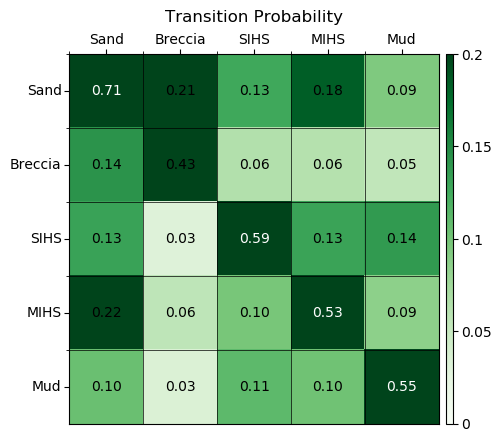
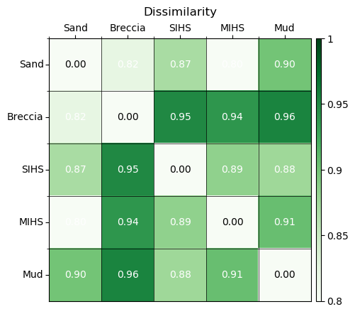
class pygeostat.categorical.TransitProb(data, sigdigs=3)¶

Calculate the transition probability matrix of categories, which are output as the DataFrame attribute self.tprob. Also output the symmetric dissimilarity matrix that is associated with the transition probabilities. This is output as the attribute self.dissim. Consider using the class functions self.plot_tprob, self.plot_dissim and self.plot_mds to display the results.

Parameters:	data (DataFile) – data.dh, data.z and data.cat must be initialized. data.catdict may also be initialized to avoid generic labels. sigdigs (round) – round the annotations to this number of decimals

Workflow Example:

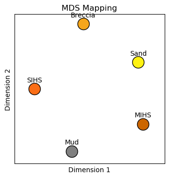
import pygeostat as gs

# Set a default categorical dictionary and colormap
gs.gsParams['data.catdict'] = {1:'Sand', 2:'Breccia', 3:'SIHS', 4:'MIHS', 5:'Mud'}
gs.gsParams['plotting.cmap_cat'] = {1:[ 1., 0.95, 0.07],
                                    2:[0.96, 0.65, 0.11],
                                    3:[0.98, 0.43, 0.09],
                                    4:[0.8, 0.4, 0.],
                                    5:[0.5, 0.5,0.5]}

# Load the data, which automatically registers the cat attribute
data = gs.ExampleData('point3d_ind_mv')

# Calculate the transition probability
transitprob = gs.TransitProb(data)

# Plot the transition probability
transitprob.plot(vlim=(0, .2))

# Plot the dissimilarity matrix and associated MDS mapping
transitprob.plot_dissim(vlim=(.8, 1))
transitprob.plot_mds(vpad=.05, figsize=(4, 4))

Code author: Ryan Barnett 2018-04-25

Plot Transition Probability Matrix¶

TransitProb.plot(vlim=(0, 1), cmap='Greens', annot_clr={0.0: 'black', 0.5: 'white'}, cbar=True, cbar_label=None, title='Transition Probability', ax=None, figsize=None, pltstyle=None)¶

Plot the transition probability matrix of categories.

Parameters:	vlim (tuple) – vlim for the data on the corrmat cmap (str) – valid Matplotlib colormap annot_clr (dict) – Indicate the text color that should be used for annotation. Values greater than annotate.keys() (cutoff), are colored by the corresponding annotate.values(). E.g., annot_clr = {-1.0e21:’black’, 0.5:’white’} cbar (bool) – Indicate if a colorbar should be plotted or not cbar_label (str) – label for the colorbar title (str) – title for the matrix ax (mpl.axis) – Matplotlib axis figsize (tuple) – Figure size (width, height) pltstyle (str) – Use a predefined set of matplotlib plotting parameters as specified by gs.gsPlotStyle. Use `False` or `None` to turn it off returnmat (bool) – return the calculated matrix
Returns:	transition probability matrix
Return type:	tprob (np.ndarray)

Code author: Ryan Barnett 2018-04-25

Plot Dissimilarity¶

TransitProb.plot_dissim(vlim=(0, 1), cmap='Greens', annot_clr={0.0: 'black', 0.5: 'white'}, cbar=True, cbar_label=None, title='Dissimilarity', ax=None, figsize=None, pltstyle=None)¶

Plot the dissim matrix of categories.

Parameters:

vlim (tuple) – vlim for the data on the corrmat
cmap (str) – valid Matplotlib colormap
annot_clr (dict) – Indicate the text color that should be used for annotation. Values greater than annotate.keys() (cutoff), are colored by the corresponding annotate.values(). E.g., annot_clr = {-1.0e21:’black’, 0.5:’white’}
cbar (bool) – Indicate if a colorbar should be plotted or not
cbar_label (str) – label for the colorbar
title (str) – title for the matrix
ax (mpl.axis) – Matplotlib axis
figsize (tuple) – Figure size (width, height)
pltstyle (str) – Use a predefined set of matplotlib plotting parameters as specified by gs.gsPlotStyle. Use False or None to turn it off

Plot MDS¶

TransitProb.plot_mds(cmap_cat=None, s=300, vpad=0, title='MDS Mapping', ax=None, figsize=None)¶

Convert self.dissim into a 2-D multidimensional scaling (MDS) mapping.

Parameters:

cmap_cat (dict) – dictionary of category colors, formmated as {catcode: catcolor}, where the catcodes must align with the keys of self.catdict. If None, drawn from gsParams[‘plotting.cmap_cat’] if its keys align with self.catdict.
s (float) – size of scatter
vpad (string or tuple) – vertical distance between the scatter and label
title (str) – title of the mapping
ax (mpl.axis) – Matplotlib axis
figsize (tuple) – Figure size (width, height)

Categorical Utilities¶

Proportion Targets¶

pygeostat.categorical.proptarget(dataprops, simprops, tol=0.0001, maxiter=100000)¶

Given the category proportions of a representative data distribution and model realizations, calculate the target proportions of each realization so that they average as a set to the representative data proportions, while preserving the variability and rank order of their existing proportions (as near as possible). Valid output proportions are ensured, where each realization sums to 1.

Parameters:	dataprops (list or np.ndarray or pd.DataFrame) – ncat global representative proportions simprops (np.ndarray or pd.DataFrame) – nreal x ncat proportions of each realization tol (float) – minimum difference that is required between the global representative proportions and the associated average proportion of the realizations. This tolerance is used as stopping criteria for the iterative algorithm. maxiter (int) – the maximum number of iterations, which is used as stopping criteria in the event that the minimum tolerance is not reached.
Returns:	output target proportions of each realization, which matches the input dimension and type of simprops.
Return type:	targetprops (np.ndarray or pd.DataFrame)

Code author: Ryan Barnett 2018-04-25

Merge Models¶

pygeostat.categorical.mergemod(catcodes, simcat, simvars)¶

Function that mimics the CCG mergemod program, allowing for simulated variables of each simulated category (existing in separate arrays) to be merged into a single array. The function only operates on one realization at a time currently, intending to be executed in a loop. Null values are assumed to be specified as nans.

Parameters:	catcodes (list) – category codes in simcat, which are provided so that they do not need to be queried for each function call simcat (DataFile or pd.DataFrame) – data with the simulated categories. If a DataFile is provided for this array, it is assumed that a dictionary of DataFiles are provided for simvars (and vice versa). simvars (ncat-dictionary) – dictionary that is formatted as {catcode: data}, where all catcodes should be present as keys, and the data must be a pd.DataFrame or gs.DataFile in correspondence with the format of simcat. The number of columns should align between the arrays, while thenumber of rows should align with simcat.
Returns:	sim – data containing the simulated category in the first column, and the variables in the remaining column. A DataFile or DataFrame is returned in correspondence with the simcat type.
Return type:	DataFile or pd.DataFrame

Code author: Ryan Barnett - 2018-03-26