Statistics¶

Collection of tools for calculating statistics.

CDF¶

Cumulative Distribution Function¶

pygeostat.statistics.cdf.cdf(var, wt=None, lower=None, upper=None, bins=None)¶

Calculates an empirical CDF using the standard method of the midpoint of a histogram bin. Assumes that the data is already trimmed or that iwt=0 for variables which are not valid.

If ‘bins’ are provided, then a binned histogram approach is used. Otherwise, the CDF is constructed using all points (as done in GSLIB).

Notes

‘lower’ and ‘upper’ limits for the CDF may be supplied and will be returned appropriately

Parameters:

var (array) – Array passed to the cdf function
wt (str) – column where the weights are stored
Lower (float) – Lower limit
upper (float) – Upper Limit
bins (int) – Number of bins to use

Returns:

midpoints (np.ndarray) – array of bin midpoints
cdf (np.ndarray) – cdf values for each midpoint value

wtpercentile¶

pygeostat.statistics.cdf.wtpercentile(cdf_x, cdf, percentile)¶: Given ‘x’ values of a CDF and corresponding CDF values, find a given percentile. Percentile may be a single value or an array-like and must be in [0, 100] or CDF bounds

z_percentile¶

pygeostat.statistics.cdf.z_percentile(z, cdf_x, cdf)¶: Given ‘cdf_x` values of a CDF and corresponding cdf values, find the percetile of a given value z. Percentile may be a single value or an array-like and must be in [0, 100] or CDF bounds.

Discretize CDF¶

pygeostat.statistics.cdf.discretize_cdf(nthresholds, data, wt=None, lower=None, upper=None)¶

Function to discretize a the cdf of the given dataset by equal probability intervals producing the midpoint x and y locations and the threshold value for each of the bins.

Notes

Functionality for choosing the thresholds should be added in the future, eg. a parameter thresholds containing a list of thresholds and then return the coordinates of the midpoints and y-values for the thresholds

Parameters:	nthresholds (int) – number of thresholds to generate, equally spaced in probability data (np.ndarray) – an array of data from which to build the cdf wt (np.ndarray) – weights to consider for building the cdf lower (float) – lower trimming value upper (float) – upper trimming value
Returns:	mp_x, mp_y, zc_x, zc_y – lists of x and y coordinates for the midpoints (mp) and threshold (zc) for each bin
Return type:	list

Examples

Discretize the cdf with 16 thresholds:

>>> (mp_x, mp_y), (cutoff_x, cutoff_y) = gs.discretize_cdf(16, df.data['Zn'])

Plot the cdf using gs.histplt:

>>> ax = gs.histplt(df.data['Zn'], icdf=True, figsize=(5, 4), xlim=(0, 60))

Plot the cutoff points on the cdf:

>>> ax.scatter(cutoff_x, cutoff_y, marker='+', s=10, lw=0.5, c='red')

Add some lines to show where the bins fall on the x-axis:

>>> for cutoff, yval in zip(cutoff_x, cutoff_y):
...     ax.vlines(cutoff, 0, yval, colors='r', lw=0.25)
...     ax.text(cutoff-0.1, yval + 0.001, round(cutoff,2), va='bottom', ha='right',
...             fontsize=8)

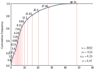
Code author: Ryan Martin - 2017-03-26

Smooth CDF¶

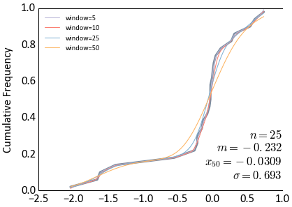
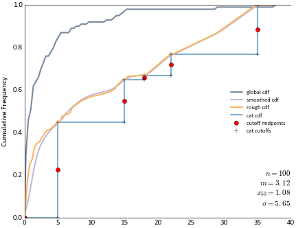
pygeostat.statistics.cdf.smooth_cdf(global_data, weights=None, ik_cdf_x=None, ik_cdf_y=None, lower=None, upper=None, nbins=500, windowfrac=None)¶

This function smooths the cdf of the given dataset using convolution with the given windowfrac parameter. Optionally a local cdf can be passed, and the smoothed distribution will be interpolated between the given cutoffs obtained from the ik3d distribution.

Parameters:	global_data (np.ndarray) – number of thresholds to generate, equally spaced in probability weights (np.ndarray) – weights for the global distribution, e.g. declustering weights ik_cdf_x (np.ndarray, optional) – cdf x-values corresponding to the output from `cdf` for a distribution to smooth the global data too, e.g. interpolate the global to the MIK cutoffs ik_cdf_y (np.ndarray, optional) – cdf y-values corresponding to the output from `cdf` for a distribution to smooth the global data too, e.g. interpolate the global to the MIK cutoffs lower (float) – the lower trimming limit for global_data; values below are omitted upper (float) – the upper trimming limit for global_data; values above are omitted nbins (int) – the number of interpolated values to return windowfrac (float) – the fraction of the total number of bins used in the window, e.g. 50% for nbins = 100 means that the window size is 50 function (string) – permissable scipy.interpolate.Rbf functions, e.g. `'linear'`, `'cubic'`, `'multiquadric'`
Returns:	x, y – lists of x, y coordinates defining the CDF for the given nbins
Return type:	list

Examples

Make some noisy data and smooth the CDF

>>> dataset = np.random.randn(100) + np.random.rand(100) * 0.5
>>> ax = gs.histplt(dataset, icdf=True)
>>> colors = gs.get_palette('cat_pastel', 6).colors[2:]
>>> for i, window in enumerate([5, 10, 25, 50]):
...     smoothx, smoothy = gs.smooth_cdf(dataset, windowfrac=window)
...     ax.plot(smoothx, smoothy, c=colors[i], lw=0.5, label='window=%i' % window)
>>> ax.legend(loc='upper left', prop={'size':5})

Try again with an example of MIK intervals and interpolating a CDF to the thresholds

>>> ax = gs.histplt(dataset, icdf=True, label='global cdf', figsize=(5,4), lower=0,
...                 bins=100)
>>> probs = np.array([0, 0.45, 0.65, 0.67, 0.77, 1.0])
>>> zvals = np.array([0, 5, 15, 18, 22, 35])
>>> itpx, itpy = gs.smooth_cdf(dataset, ik_cdf_x=zvals, ik_cdf_y=probs, nbins=100, lower=0,
...                            windowfrac=0)
>>> smoothx, smoothy = gs.smooth_cdf(dataset, ik_cdf_x=zvals, ik_cdf_y=probs, nbins=100,
...                                  lower=0, windowfrac=7)
>>> # local indicator CDF
>>> pts, ipts = gs.build_indicator_cdf(probs, zvals)
>>> ax.scatter(ipts[:, 0], ipts[:, 1], c='red', marker='o', label='cutoff midpoints')
>>> ax.scatter(pts[:, 0], pts[:, 1], c='black', marker='+', label='cat cutoffs', zorder=5)
>>> ax.plot(smoothx, smoothy, c=colors[0], label='smoothed cdf')
>>> ax.plot(itpx, itpy, c=colors[3], label='rough cdf')
>>> ax.plot(pts[:, 0], pts[:, 1], c=colors[2], zorder=0, label='cat cdf')
>>> ax.set_xbound(lower=0)
>>> ax.set_ybound(lower=0, upper=1)
>>> ax.legend(loc='center right', prop={'size': 6})

Code author: Ryan Martin - 2017-04-17

Build Indicator CDF¶

pygeostat.statistics.cdf.build_indicator_cdf(prob_ik, zvals)¶

Build the X-Y data required to plot a categorical cdf

Parameters:	prob_ik (np.ndarray) – the p-vals corresponding to the cutoffs zvals (np.ndarray) – the corresponding z-value specifying the cutoffs
Returns:	points, midpoints – the x and y coordinates of (1) the cutoffs and (2) the midpoints for each cutoff
Return type:	np.ndarray

Code author: Ryan Martin - 2017-04-17

Variance From CDF¶

pygeostat.statistics.cdf.variance_from_cdf(cdfx, cdfy, nsample=1000)¶: Compute the variance by randomly sampling the cdf brute force

Stdev From CDF¶

pygeostat.statistics.cdf.stdev_from_cdf(cdfx, cdfy, nsample=1000)¶: Compute the stdsev of the cdf from a n-sample sized random sample from the cdf

Kernel Density Estimation Functions¶

Univariate KDE with StatsModels¶

pygeostat.statistics.kde.kde_statsmodels_u(x, x_grid, bandwidth=0.2, **kwargs)¶: Univariate Kernel Density Estimation with Statsmodels

Multivariate KDE with StatsModels¶

pygeostat.statistics.kde.kde_statsmodels_m(x, x_grid, bandwidth=0.2, **kwargs)¶: Multivariate Kernel Density Estimation with Statsmodels

KDE with Scikit-learn¶

pygeostat.statistics.kde.kde_sklearn(x, x_grid, bandwidth=0.2, **kwargs)¶: Kernel Density Estimation with Scikit-learn

KDE with Scipy¶

pygeostat.statistics.kde.kde_scipy(x, x_grid, bandwidth=0.2, **kwargs)¶: Kernel Density Estimation based on different packages and different kernels Note that scipy weights its bandwidth by the covariance of the input data. To make the results comparable to the other methods, we divide the bandwidth by the sample standard deviation here.

Weighted Statistics¶

Weighted Mean¶

pygeostat.statistics.utils.weightedmean(x, wt)¶: Calculates the weighted mean

Weighted Variance¶

pygeostat.statistics.utils.weightedvar(x, wt)¶: Calculates the weighted variance

Weighted Correlation¶

pygeostat.statistics.utils.weightedcorr(x, y, wt)¶: Calculates the weighted correlation

Weighted Rank Correlation¶

pygeostat.statistics.utils.weightedcorr_rank(x, y, wt)¶: Calculatees the weighted spearman rank correlation

Weighted Covariance¶

pygeostat.statistics.utils.weightedcov(x, y, wt)¶: Calculates the weighted covariance

Weighted Skew¶

pygeostat.statistics.utils.weightedskew(x, wt)¶: Calculates the weighted skewness

Assorted Stats Functions¶

Nearest Positive Definite Correlation Matrix¶

pygeostat.statistics.utils.nearpd(inmat)¶

This function uses R to calculate the nearest positive definite matrix within python. An installation of R with the library “Matrix” is required. The module rpy2 is also needed

The only requirement is an input matrix. Can be either a pandas dataframe or numpy-array.

Parameters:	inmat (np.ndarray, pd.DataFrame) – input numpy array or pandas dataframe, not numpy matrix
Returns:	pdmat – Nearest positive definite matrix as a numpy-array
Return type:	np.ndarray

Code author: Warren Black - 2015-08-02

Accuracy Plot Statistics - Simulation¶

pygeostat.statistics.utils.accsim(truth, reals, pinc=0.05)¶

Calculates the proportion of locations where the true value falls within symmetric p-PI intervals when completing a jackknife study. A portion of the data is excluded from the conditioning dataset and the excluded sample locations simulated values are then checked.

Accuracy Plot Statistics - CDF thresholds¶

pygeostat.statistics.utils.accmik(truth, thresholds, mikprobs, pinc=0.05)¶

Similar to accsim but accepting mik distributions instead

Mostly pulled from accsim

Parameters:

truth (np.ndarray) – Tidy (long-form) 1D data where a single column containing the true values. A pandas dataframe/series or numpy array can be passed
thresholds (np.ndarray) – 1D array of thresholds where each CDF is defined by these thresholds and the probability given in the mikprobs array for each location.
mikprobs (np.ndarray) – Tidy (long-form) 2D data where a single column contains values from a single MIK cutoff and each row contains the simulated values for the corresponding single truth location. A pandas dataframe or numpy matrix can be passed
pinc (float) – Increments between the probability intervals to calculate within (0, 1)

Returns:

propavg (pd.DataFrame) – Dataframe with the calculated probability intervals and the fraction within the interval
sumstats (dict) – Dictionary containing the average variance (U), mean squared error (MSE), accuracy measure (acc), precision measure (pre), and a goodness measure (goo)

Code author: Warren Black and Ryan Martin - 2017-04-17

PostSim¶

pygeostat.statistics.postsim.postsim_multfiles(file_base_or_list, output_name, Nr=None, file_ending=None, fltype=None, output_fltype=None, zero_padding=0, variables=None, var_min=None)¶

The multiple file postsim function uses recursive statistics for memory management and coolness factor. See http://people.revoledu.com/kardi/tutorial/RecursiveStatistic/ This function will take multiple realizations and post process the results into mean and variance for each variable. You can either pass it a list of files to iterate through or a filebase name and the number of realizations.

Parameters:

file_base_or_list (list) or (str) – List of files or path + base name of sequentially named files
output_name (str) – ath (or name) of file to write output to.
Nr (int) – Number of realizations. Needed if file base name is passed.
file_ending (str) – file ending (ex. “out”). Used if file base name is passed. Period is not included.
fltype (str) – Type of data file: either csv, gslib, hdf5, or gsb. Used if file base name is passed and file_ending is not used.
output_fltype (str) – Type of output data file: either csv, gslib, hdf5, or gsb.
zero_padding (int) – Number of zeros to padd number in sequentially named files with. Default is 0.
variables (str) – List of variables to process.
var_min (list) or (float) – Minimum trimming limit to use. If one value is passed it will apply the trimming limit to all variables. Or a list of trimming limit for each variable can be passed.

Code author: Tyler Acorn - 2016-08-03