Introduction to Python and pygeostat¶

Introduction¶

This documentation gives a brief overview of python for researchers and affiliates of CCG. This documentation is not an introduction to python in general, but is designed to help with:

deciding whether using python would be valuable for your work
applying python to geostatistics problems using CCG and GSLIB software
the basics of using python and pygeostat to analyze data, visualize results and interface with Paraview

Python is an interpreted, high level general purpose programming and scripting language which is very well suited to many of the common scripting tasks where bash or matlab would typically be used, and many tasks where an entire Fortran program might have previously been used. The huge collection of libraries for python covering machine learning, statistics, data management and optimization make it very useful for geostatistical workflows. There are many excellent tutorials for Python 3 available (http://docs.python.org/3/tutorial/introduction.html) which do a much better job introducing the language than I would.

Pygeostat is a python module using fortran libraries which was written to facilitate working with GeoEAS data files (GSLIB format), CSV data files, and GSLIB and CCG software. The integrated fortran libraries making pygeostat extremely quick to use for many applications, such as variogram calculation and modeling requiring no parameter files. For other GSLIB and CCG programs, generic interface routines are provided to interface with the programs using standard string interpolation techniques familiar to anyone who has scripted with Bash.

Loading Modules¶

The following code section is normally used as a header for scripts using pygeostat. pygeostat is imported as well as the python math package numpy and data analysis package pandas. The standard python plotting library matplotlib is imported. The %inline option is used to include figures in this documentation rather than saving images separately.

'''pygeostat_examples.ipynb: Demonstrate usage of pygeostat'''
__author__ = 'Jared Deutsch'
__date__ = '2015-11-04'
__version__ = '4.0'

import pygeostat as gs
import numpy as np
import pandas as pd
import matplotlib.pyplot as plt
%matplotlib inline

Super quick introduction to python for CCG researchers¶

An extremely quick introduction to python is given here. Python is a high level interpreted programming language. Variable assignment and math is simple. The print operator prints to the screen. Whitespace (in the form of 4 spaces) is used for blocks such as if statements, or loops.

print('Hello World!')

print('Math is easy and works as expected')
a = 1
b = 2
print('a =',a,'b =',b)
print('a + b =',a+b)
print('a/b+0.2 =',a/b+0.2)

if (1>2):
    print('This statement is unreachable')
else:
    print('Note the 4 spaces for block statements like if and loops')

print('Loops can use a list, or a range among other things!')
for i in [1,2,10]:
    print(i)

print('Note that everything starts from 0 in python unlike Fortran')
for i in range(3):
    print(i)

mystr = 'Hello World!'
print('Lots of helpful options are built in such as string splitting:',mystr.split())

Hello World!
Math is easy and works as expected
a = 1 b = 2
a + b = 3
a/b+0.2 = 0.7
Note the 4 spaces for block statements like if and loops
Loops can use a list, or a range among other things!
1
2
10
Note that everything starts from 0 in python unlike Fortran
0
1
2
Lots of helpful options are built in such as string splitting: ['Hello', 'World!']

Importing GSLIB files to python with pygeostat¶

We will use the oilsands.dat training data set for this example. A pygeostat DataFile object is used to store the data, and relevant parameters such as the names of x, y and z coordinates. The DataFile class stores data by default in a Pandas DataFrame called ‘data’. Pandas provides the ‘head()’ function to print the first few rows of a DataFrame - we can see that the oilsands data is read in to this object.

datafl = gs.DataFile(flname='../../examples/data/oilsands.dat',
                     dh='Drillhole Number',x='East',y='North',z='Elevation')
datafl.data.head()

	Drillhole Number	East	North	Elevation	Bitumen	Fines	Chlorides	Facies Code
0	2	1245	10687.09	257.5	7.378	28.784	-9	-9
1	2	1245	10687.09	254.5	9.176	22.897	-9	-9
2	2	1245	10687.09	251.5	11.543	15.144	-9	-9
3	2	1245	10687.09	248.5	6.808	30.598	-9	-9
4	2	1245	10687.09	245.5	10.657	18.011	-9	-9

There are a number of special variables in the DataFile class including the drillhole identifier (dh), and coordinates x, y and z. These can be accessed by name, or number. Recall that as python uses zero-ordering (the same as C and C++), column 1 in python refers to column 2 in GSLIB/Fortran one-ordering.

print('\nFirst couple rows of Z:\n', datafl.data[datafl.z].head())
print('\nFirst couple rows of DH:\n', datafl.data['Drillhole Number'].head())
print('\nFirst couple rows of the second column: (column 2 if GSLIB/Fortran 1 ordered or 1'
      ' if Python/C/C++ 0 ordered)\n', datafl.data.icol(1).head())

First couple rows of Z:
  257.5
  254.5
  251.5
  248.5
  245.5
Name: Elevation, dtype: float64

First couple rows of DH:
  2
  2
  2
  2
  2
Name: Drillhole Number, dtype: int64

First couple rows of the second column: (column 2 if GSLIB/Fortran 1 ordered or 1 if Python/C/C++ 0 ordered)
  1245
  1245
  1245
  1245
  1245
Name: East, dtype: float64

pygeostat provides a number of convenience functions which can be used. Slicing is easy and unique categories can be identified.

print('\nUnique categories can be identified, for example facies code:')
print(datafl.unique_cats('Facies Code'))

print('\nSlicing can be done as well, for example data in drill hole 3:')
print(datafl.data[datafl.data['Drillhole Number'] == 3])

print('\nThe bitumen and fines content for fines greater than 40 (first few rows)')
print(datafl.data[['Bitumen','Fines']][datafl.data['Fines'] > 40.0].head())

print('Creating new columns is simple, for example bitumen * fines - 200:')
datafl.data['Bitumen times Fines minus 200'] = datafl.data['Bitumen']*datafl.data['Fines']-200
print(datafl.data.head())

Unique categories can be identified, for example facies code:
[-9, 23, 30, 31, 40, 50, 60, 61, 69, 70]

Slicing can be done as well, for example data in drill hole 3:
    Drillhole Number    East    North  Elevation  Bitumen   Fines  Chlorides  18                 3  1262.5  10821.3      242.5   11.378  15.659         -9
19                 3  1262.5  10821.3      239.5   12.436  12.163         -9
20                 3  1262.5  10821.3      236.5    8.900  23.700         -9
21                 3  1262.5  10821.3      233.5    8.870  23.837         -9
22                 3  1262.5  10821.3      230.5    9.733  21.057         -9
23                 3  1262.5  10821.3      227.5   10.984  16.931         -9
24                 3  1262.5  10821.3      224.5   11.113  16.549         -9
25                 3  1262.5  10821.3      221.5    9.054  23.551         -9
26                 3  1262.5  10821.3      218.5   15.029   5.716         -9
27                 3  1262.5  10821.3      215.5   12.957  10.565         -9
28                 3  1262.5  10821.3      212.5   13.589   8.537         -9

    Facies Code
18           -9
19           -9
20           -9
21           -9
22           -9
23           -9
24           -9
25           -9
26           -9
27           -9
28           -9

The bitumen and fines content for fines greater than 40 (first few rows)
    Bitumen   Fines
54    2.900  43.500
73    2.465  44.838
74    0.000  52.900
75    0.000  52.900
76    0.000  52.900
Creating new columns is simple, for example bitumen * fines - 200:
   Drillhole Number  East     North  Elevation  Bitumen   Fines  Chlorides  0                 2  1245  10687.09      257.5    7.378  28.784         -9
1                 2  1245  10687.09      254.5    9.176  22.897         -9
2                 2  1245  10687.09      251.5   11.543  15.144         -9
3                 2  1245  10687.09      248.5    6.808  30.598         -9
4                 2  1245  10687.09      245.5   10.657  18.011         -9

   Facies Code  Bitumen times Fines minus 200
0           -9                      12.368352
1           -9                      10.102872
2           -9                     -25.192808
3           -9                       8.311184
4           -9                      -8.056773

Getting basic statistics from the data set can be done using the describe command - here just bitumen and fines are summarized:

datafl.data[['Bitumen','Fines']].describe()

	Bitumen	Fines
count	5808.000000	5808.000000
mean	7.708852	28.707298
std	5.136709	21.247085
min	0.000000	0.861000
25%	2.877750	10.166000
50%	7.480000	24.453000
75%	12.666000	42.823250
max	18.428000	86.777000

Correlation matrix:

datafl.data[['Bitumen','Fines']].corr()

	Bitumen	Fines
Bitumen	1.000000	-0.843863
Fines	-0.843863	1.000000

Conditionally setting data in Pandas requires indexing the location in the array:

# Set all facies -9 values to -999 values
datafl.data.loc[datafl.data['Facies Code'] == -9,'Facies Code'] = -999
datafl.data.head()

	Drillhole Number	East	North	Elevation	Bitumen	Fines	Chlorides	Facies Code	Bitumen above 7
0	2	1245	10687.09	257.5	7.378	28.784	-9	-999	1
1	2	1245	10687.09	254.5	9.176	22.897	-9	-999	1
2	2	1245	10687.09	251.5	11.543	15.144	-9	-999	1
3	2	1245	10687.09	248.5	6.808	30.598	-9	-999	0
4	2	1245	10687.09	245.5	10.657	18.011	-9	-999	1

Saving data to CSV and VTK file formats¶

Working with data is only useful if it can be saved. Here, the data is re-imported to get rid of the changes to the data set.

datafl = gs.DataFile(flname='../../examples/data/oilsands.dat', dh='Drillhole Number', x='East',
                     y='North', z='Elevation')

We can create an indicator column which is 1 where the bitumen is above 7% and 0 otherwise.

datafl.data['Bitumen above 7'] = np.zeros(len(datafl.data['Bitumen']))
datafl.data.loc[datafl.data['Bitumen'] >= 7.0,'Bitumen above 7'] = 1
datafl.data[['Bitumen','Bitumen above 7']].head()

	Bitumen	Bitumen above 7
0	7.378	1
1	9.176	1
2	11.543	1
3	6.808	0
4	10.657	1

This file can be saved as a GSLIB file or as a CSV file which can be opened by Excel.

outgslibfl = 'oilsands_out.dat'
outcsvfl = 'oilsands_out.csv'

datafl.writefile(flname=outgslibfl, fltype='GSLIB')

The datafile can be saved as a GSLIB file: oilsands_out.dat

Or as a CSV file which can be opened by Excel A subset of columns, can be saved with any of these modes - just saving X, Y and Z for example: oilsands_out.csv

datafl.writefile(flname=outcsvfl, variables=['East','North','Elevation'], fltype='CSV')

A VTK file can also be created for visualization with Paraview. This requires the DataFile class to have the X, Y and Z coordinates (.x, .y and .z attributes)

outvtkfl = 'oilsands_out.vtk'
datafl.writefile(flname=outvtkfl, fltype='VTK')

The datafile can be saved as a VTK file: oilsands_out.vtk

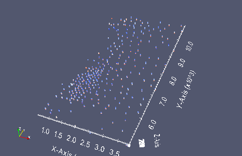
A small screen capture from paraview of the oil sands data points

from IPython.display import Image
datavtk = Image(filename='oilsands_vtk.png')
datavtk

Python Classes¶

Class objects can be viewed as a container for a structured set of variables and functions. As a result of the controlled structure where variables containing data or parameters are saved in specific format, to a specific variable, functions can be used in a semi-automatic fashion. As such, work flows can be greatly simplified by using classes!

Within the code of classes, variables stored within the class are initialized as self.<variable>. The self name space tells python that the variable should remain accessible to the user and any other functions within the class. These self variables stored within the class can be any permissible python object; which includes but is not limited to: string, list, dictionary, pandas dataframe, float, integer, ect.

As an example, we’ve already started a gs.DataFile class above with the oilsands.dat training data set, saved as datafl.

On the user-end, to call the data stored within the datafl variogram class, you would replace self with data. For example, let check out the the first few lines that were loaded from the data file:

datafl.data.head()

	Drillhole Number	East	North	Elevation	Bitumen	Fines	Chlorides	Facies Code	Bitumen above 7
0	2	1245	10687.09	257.5	7.378	28.784	-9	-9	1
1	2	1245	10687.09	254.5	9.176	22.897	-9	-9	1
2	2	1245	10687.09	251.5	11.543	15.144	-9	-9	1
3	2	1245	10687.09	248.5	6.808	30.598	-9	-9	0
4	2	1245	10687.09	245.5	10.657	18.011	-9	-9	1

Within the source code for gs.DataFile, the column IDs for the x, y, and z data are saved within the class as they were specified when it was created. To view what they are you can call them as:

print('The x data column ID is: ', datafl.x)
print('The y data column ID is: ', datafl.y)
print('The z data column ID is: ', datafl.z)

The x data column ID is:  East
The y data column ID is:  North
The z data column ID is:  Elevation

Much like variables are stored within the class, so are functions unique to the class. Meaning they are only accessible by the class object. So like you would call a stored variable, you call functions as an extension of the variogram class name space. For example, when using a gs.Variogram, you can calculate the experimental variograms by calling:

vario.varcalc()

Within pygestat there are numerous classes set-up. These include:

gs.DataFile

gs.GridDef

gs.Variogram

gs.VariogramModel

gs.Program

Using python + pygeostat for GSLIB scripting¶

Python (and pygeostat to make things easier) can be used for scripting together GSLIB and CCG programs. Normally we would use bash for scripts, but python is very useful for complicated scripts, particularly for visualization and keeping track of numerous domains, variables and data files. Python can also be used to call bash scripts or execute shell code (and vice versa).

The standard method for running a GSLIB program with python + pygeostat is to create a GSLIBProgram class for each program that will be used. We can create a string with variables (such as {datafl}) which can then be interpolated. A small example:

histpltpar = '''                  Parameters for HISTPLT
                  **********************

START OF PARAMETERS:
{datafl}          -file with data
{varcol}   0                        -   columns for variable and weight
-1.0     1.0e21              -   trimming limits
{outfl}                   -file for PostScript output
 0.0      -20.0               -attribute minimum and maximum
-1.0                         -frequency maximum (<0 for automatic)
20                           -number of classes
0                            -0=arithmetic, 1=log scaling
0                            -0=frequency,  1=cumulative histogram
0                            -   number of cum. quantiles (<0 for all)
3                            -number of decimal places (<0 for auto.)
{varname}                                                    -title
1.5                          -positioning of stats (L to R: -1 to 1)
-1.1e21                      -reference value for box plot
'''

histplt = gs.Program(program='histplt', parfile='histplt.par')

print('Basic operations like calling programs with string interpolation is fast')
print('A convenience "GSCOL" function is provided for getting the column given a name')
histplt.run(parstr=histpltpar.format(datafl=datafl.flname,varcol=datafl.gscol('Bitumen'),
    varname='Bitumen',outfl='histplt_bitumen.ps'))

Basic operations like calling programs with string interpolation is fast
A convenience "GSCOL" function is provided for getting the column given a name
Calling:  ['histplt', 'histplt.par']

HISTPLT Version: 2.905

 data file = ../../examples/data/oilsands.dat
 columns =           5           0
 trimming  limits =       -1.000000    1.000000E+21
 output file = histplt_bitumen.ps
 attribute limits =    0.000000E+00      -20.000000
 frequency  limit =       -1.000000
 number of classes =          20
 log scale option =           0
 cumulative frequency option =           0
 number of decimal places =           3
 title = Bitumen
 position of stats =        1.500000
 reference value =   -1.100000E+21

There are     5808 data with:
  mean value          =      7.70886
  median value        =      7.48000
  standard deviation  =      5.13627
  minimum and maximum =       .00000    18.42800


HISTPLT Version: 2.905 Finished

Stop - Program terminated.

Parameters can also be saved in a dictionary and used that way. In addition, looping over multiple variables is easy - they can simply be referred to by name.

print('Parameters can also be saved in a dictionary and used that way')
mypars = {'datafl':datafl.flname,
            'varcol':datafl.gscol('Fines'),
            'varname':'Fines',
            'outfl':'histplt_fines.ps'}
histplt.run(parstr=histpltpar.format(**mypars))

print('Looping over multiple variables is easy with this approach')
for variable in ['Bitumen','Fines']:
    mypars = {'datafl':datafl.flname,
            'varcol':datafl.gscol(variable),
            'varname':variable,
            'outfl':'histplt_'+variable+'.ps'}
    histplt.run(parstr=histpltpar.format(**mypars))

Parameters can also be saved in a dictionary and used that way
Calling:  ['histplt', 'histplt.par']

HISTPLT Version: 2.905

 data file = ../../examples/data/oilsands.dat
 columns =           6           0
 trimming  limits =       -1.000000    1.000000E+21
 output file = histplt_fines.ps
 attribute limits =    0.000000E+00      -20.000000
 frequency  limit =       -1.000000
 number of classes =          20
 log scale option =           0
 cumulative frequency option =           0
 number of decimal places =           3
 title = Fines
 position of stats =        1.500000
 reference value =   -1.100000E+21

There are     5808 data with:
  mean value          =     28.70733
  median value        =     24.45354
  standard deviation  =     21.24525
  minimum and maximum =       .86100    86.77700


HISTPLT Version: 2.905 Finished

Stop - Program terminated.


Looping over multiple variables is easy with this approach
Calling:  ['histplt', 'histplt.par']

HISTPLT Version: 2.905

 data file = ../../examples/data/oilsands.dat
 columns =           5           0
 trimming  limits =       -1.000000    1.000000E+21
 output file = histplt_Bitumen.ps
 attribute limits =    0.000000E+00      -20.000000
 frequency  limit =       -1.000000
 number of classes =          20
 log scale option =           0
 cumulative frequency option =           0
 number of decimal places =           3
 title = Bitumen
 position of stats =        1.500000
 reference value =   -1.100000E+21

There are     5808 data with:
  mean value          =      7.70886
  median value        =      7.48000
  standard deviation  =      5.13627
  minimum and maximum =       .00000    18.42800


HISTPLT Version: 2.905 Finished

Stop - Program terminated.


Calling:  ['histplt', 'histplt.par']

HISTPLT Version: 2.905

 data file = ../../examples/data/oilsands.dat
 columns =           6           0
 trimming  limits =       -1.000000    1.000000E+21
 output file = histplt_Fines.ps
 attribute limits =    0.000000E+00      -20.000000
 frequency  limit =       -1.000000
 number of classes =          20
 log scale option =           0
 cumulative frequency option =           0
 number of decimal places =           3
 title = Fines
 position of stats =        1.500000
 reference value =   -1.100000E+21

There are     5808 data with:
  mean value          =     28.70733
  median value        =     24.45354
  standard deviation  =     21.24525
  minimum and maximum =       .86100    86.77700


HISTPLT Version: 2.905 Finished

Stop - Program terminated.

Grid definitions can be used the same way as other parameters, ie: a string that we interpolate into parameter files, but saving it as a pygeostat GridDef class helps with saving out the file as a VTK file for visualization with paraview. An example using the grid definition class and calling kt3dn:

gridstr = '''35 500.  100.      -nx, xmin, xsize
      60  5000.  100.      -ny, ymin, ysize
      15   145.  10.      -nz, zmin, zsize'''

kt3dnpar = '''                 Parameters for KT3DN
                 ********************

START OF PARAMETERS:
../../examples/data/oilsands.dat
{cols}  0    -columns for DH,X,Y,Z,var,sec var
-1.0e21   1.0e21       -   trimming limits
0                            -option: 0=grid, 1=cross, 2=jackknife
NOFILE                       -file with jackknife data
1   2   0    5    0          -   columns for X,Y,Z,vr and sec var
0    100         -debugging level: 0,3,5,10; max data for GSKV
temp
{outfl}
{griddef}
4   4   4         -x,y and z block discretization
2    40              -min, max data for kriging
0      0      -max per octant, max per drillhole (0-> not used)
4000.0  4000.0  4000.0     -maximum search radii
 0.0   0.0   0.0                 -angles for search ellipsoid
1   7.71   0.6   -0=SK,1=OK,2=LVM(resid),3=LVM((1-w)*m(u))),4=colo,5=exdrift, skmean, corr
0 0 0 0 0 0 0 0 0            -drift: x,y,z,xx,yy,zz,xy,xz,zy
0                            -0, variable; 1, estimate trend
NOFILE                       -gridded file with drift/mean
4                            -  column number in gridded file
2    0.08                     -nst, nugget effect
2    0.25  40.0   0.0   0.0    -it,cc,ang1,ang2,ang3
        400.0  300.0  25.0    -a_hmax, a_hmin, a_vert
2    0.67  40.0   0.0   0.0    -it,cc,ang1,ang2,ang3
      8000.0 4500.0  30.0    -a_hmax, a_hmin, a_vert
'''

print('For grids it is useful to save the grid definition which can be loaded from a string or specified as nx=,ny=,...')
griddef = gs.GridDef(grid_str=gridstr)
print(str(griddef))
print('Values can be accessed directly using this way, for example nx =',griddef.nx)

print('This can be used for scripting, for example with kt3dn:')
kt3dn = gs.Program(program='kt3dn', parstr=kt3dnpar, parfile='kt3dn.par')
kt3dnpars ={'datafl':datafl.flname,
            'griddef':str(griddef),
            'outfl':'kt3dn.out',
            'cols':datafl.gscol([datafl.dh,datafl.x,datafl.y,datafl.z,'Bitumen'],string=True)}

print('Note that the string representation of columns can be returned using the GSCOL function for a list of variables:',
      kt3dnpars['cols'])

kt3dn.run(parstr=kt3dn.parstr.format(**kt3dnpars))

For grids it is useful to save the grid definition which can be loaded from a string or specified as nx=,ny=,...
35 500.0 100.0
60 5000.0 100.0
15 145.0 10.0
Values can be accessed directly using this way, for example nx = 35
This can be used for scripting, for example with kt3dn:
Note that the string representation of columns can be returned using the GSCOL function for a list of variables: 1 2 3 4 5
Calling:  ['kt3dn', 'kt3dn.par']

 KT3DN Version: 4.202

  data file = ../../examples/data/oilsands.dat
  columns =            1           2           3           4           5
           0
  trimming limits =  -1.0000000E+21  1.0000000E+21
  kriging option =            0
  jackknife data file = NOFILE
  columns =            1           2           0           5           0
  debugging level =            0
  debugging file = temp
  output file = kt3dn.out
  nx, xmn, xsiz =           35   500.0000       100.0000
  ny, ymn, ysiz =           60   5000.000       100.0000
  nz, zmn, zsiz =           15   145.0000       10.00000
  block discretization:           4           4           4
  ndmin,ndmax =            2          40
  max per octant =            0
  max per drillhole =            0
  search radii =    4000.000       4000.000       4000.000
  search anisotropy angles =   0.0000000E+00  0.0000000E+00  0.0000000E+00
  ktype, skmean =           1   7.710000
  drift terms =            0           0           0           0           0
           0           0           0           0
  itrend =            0
  external drift file = NOFILE
  variable in external drift file =            4
  nst, c0 =            2  7.9999998E-02
  it,cc,ang[1,2,3];            2  0.2500000       40.00000      0.0000000E+00
  0.0000000E+00
  a1 a2 a3:    400.0000       300.0000       25.00000
  it,cc,ang[1,2,3];            2  0.6700000       40.00000      0.0000000E+00
  0.0000000E+00
  a1 a2 a3:    8000.000       4500.000       30.00000
 Checking the data set for duplicates
  No duplicates found
 Data for KT3D: Variable number            5
   Number   =         5808
   Average  =    7.708860
   Variance =    26.38120
 Presorting the data along an arbitrary vector
 Data was presorted with angles:   12.50000       12.50000       12.50000
 Setting up rotation matrices for variogram and search
 Setting up super block search strategy

 Working on the kriging
   currently on estimate      3150
   currently on estimate      6300
   currently on estimate      9450
   currently on estimate     12600
   currently on estimate     15750
   currently on estimate     18900
   currently on estimate     22050
   currently on estimate     25200
   currently on estimate     28350
   currently on estimate     31500

 KT3DN Version: 4.202 Finished

Saving gridded GSLIB files in VTK format¶

Gridded files can be saved out in VTK format after loading up using pygeostat making sure to specify a grid definition.

krigedfl = gs.DataFile(flname='kt3dn.out',readfl='True',dftype='grid',
                       griddef=griddef)

After that just specify to save as VTK, same as before: kt3dn_out.vtk

krigedfl.writefile(flname='kt3dn_out.vtk',fltype='vtk')

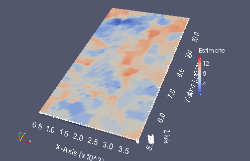
A small screen capture from paraview of the kriged grid

from IPython.display import Image
krigedvtk = Image(filename='kt3dn_vtk.png')
krigedvtk

Parallel GSLIB scripting with pygeostat¶

Running a GSLIB program in parallel using pygeostat is straight forward using a list of parameter dictionaries. Suppose we wanted histograms of bitumen, fines and chlorides for this data set. Of course, it would be faster to just run these one after another but this quick task will be used to demonstrate how parallelization with pygeostat can be used. A list of argument dictionaries is created - we specify a different parameter file name (for example histplt_bitumen.par, histplt_chlorides.par) for each variable and different parameter strings (string representations of parameter files).

There is another consideration. If GSLIB programs attempt to simultaneously open and read a file, only one process will get access to the file causing the other program calls to fail. We can get around this by specifying a “testfilename” as a parameter. Before executing each parallel process, pygeostat will attempt to open and read the file. If the file is busy, pygeostat will wait a short period to time and try again. This works in most cases, but will not work for massive data files, or programs with long run times which open a data file many times such as trans_trend.

# Create an empty list of GSLIB calling parameters, callpars
callpars = []
# For each variable we want to run in parallel, assemble a dictionary of parameters and append to callpars
for variable in ['Bitumen','Fines','Chlorides']:
    # Establish the parameter file for this variable
    mypars = {'datafl':datafl.flname,
            'varcol':datafl.gscol(variable),
            'varname':variable,
            'outfl':'histplt_'+variable+'.ps'}
    # Assemble the arguments for the GSLIB call and add the arguments to the list of calls
    callpars.append({'parstr':histpltpar.format(**mypars),
            'parfile':'histplt_'+variable+'.par',
            'testfilename':datafl.flname})

# Now we can run in parallel:
histplt = gs.Program(program='histplt', parfile='histplt.par')
gs.runparallel(histplt, callpars)

Creating parallel processes
Pool assembled, asynchronously processing
Asynchronous execution finished.

Desurveying and compositing¶

There is limited functionality in pygeostat to perform linear desurveying and compositing of raw data

# Read in the collars
collarfl = gs.DataFile(flname='./collars.csv',readfl=True,x='Easting',
                                 y='Northing',z='Elevation',dh='Drillhole')
print('Collars:\n',collarfl.data.head())
# Surveys
surveyfl = gs.DataFile(flname='./downhole.csv',readfl=True,dh='Drillhole')
print('\nSurveys:\n',surveyfl.data.head())
# Raw data file
rawdatafl = gs.DataFile(flname='./rawdata.csv',readfl=True,dh='Drillhole',
                               ifrom='From',ito='To')
print('\nRaw data file:\n',rawdatafl.data.head())

The raw data will first be composited to 15 meter lengths using the most frequent category for rock type and a linear average for grade.

comps = gs.utils.desurvey.set_comps(rawdatafl,15.0)
print('Composite lengths to use:\n',comps)
upscaled = gs.utils.desurvey.get_comps(comps,rawdatafl,{'Rock Type':'categorical',
                                               'Grade':'continuous'})
rawdatafl.origdata = rawdatafl.data.copy() # Save a copy of the original data just in case...
rawdatafl.data = upscaled # Make the upscaled data the primary data set
print('\nComposited data:\n',upscaled)

Composite lengths to use:
    Drillhole  From   To
    DH101     0   15
    DH101    15   30
    DH101    30   45
    DH101    45   60
    DH101    60   75
    DH101    75   90
    DH101    90  105
    DH102     0   15
    DH102    15   30
    DH102    30   45
   DH102    45   60
   DH102    60   75
   DH102    75   90
   DH102    90  105
   DH102   105  120
   DH102   120  135
   DH102   135  150

Composited data:
        Grade  Rock Type Drillhole  From   To
 5.370400          2     DH101     0   15
 4.765147          1     DH101    15   30
 5.151280          1     DH101    30   45
 5.127600          2     DH101    45   60
 4.936727          3     DH101    60   75
 4.376967          3     DH101    75   90
 4.437598          3     DH101    90  105
 4.876240          4     DH102     0   15
 4.926200          4     DH102    15   30
 5.072747          4     DH102    30   45
4.294660          4     DH102    45   60
5.264047          4     DH102    60   75
5.272420          3     DH102    75   90
5.004067          4     DH102    90  105
4.906380          2     DH102   105  120
4.464113          4     DH102   120  135
4.276362          3     DH102   135  150

Now these composites will be desurveyed and X,Y,Z values assigned to the midpoints of the composites.

drillholes = gs.utils.set_desurvey(collarfl,surveyfl,'Along','Azimuth','Inclination')
print('Drillhole objects are created which can be used to desurvey:')
print(drillholes['DH101'])
print(drillholes['DH102'])

Drillhole objects are created which can be used to desurvey:
Drillhole DH101 collared at (1867.0,12022.0,342.0)
Drillhole DH102 collared at (1927.0,12880.0,335.0)

gs.utils.get_desurvey(rawdatafl,drillholes,x=collarfl.x,y=collarfl.y,z=collarfl.z)
print(rawdatafl.data.head())

      Grade  Rock Type Drillhole  From  To      Easting      Northing  0  5.370400          2     DH101     0  15  1867.715534  12023.239341
1  4.765147          1     DH101    15  30  1869.369505  12025.832072
2  5.151280          1     DH101    30  45  1871.068058  12028.447613
3  5.127600          2     DH101    45  60  1872.766610  12031.063155
4  4.936727          3     DH101    60  75  1874.442209  12033.693319

    Elevation
0  334.637796
1  319.956883
2  305.284669
3  290.612455
4  275.940241

The data file has been desurveyed, last step is to convert the alphanumeric drill holes to numeric values and save it out for working with GSLIB programs.

# Convert to numeric drill hole IDs
dhdict = {'DH101':101,
          'DH102':102}
rawdatafl.applydict('Drillhole','DH',dhdict)
print(rawdatafl.data.head())
# Save out as VTK
rawdatafl.writefile(flname='desurveyed_data.vtk',variables=['Rock Type','Grade','DH'],fltype='vtk')

      Grade  Rock Type Drillhole  From  To      Easting      Northing  0  5.370400          2     DH101     0  15  1867.715534  12023.239341
1  4.765147          1     DH101    15  30  1869.369505  12025.832072
2  5.151280          1     DH101    30  45  1871.068058  12028.447613
3  5.127600          2     DH101    45  60  1872.766610  12031.063155
4  4.936727          3     DH101    60  75  1874.442209  12033.693319

    Elevation   DH
0  334.637796  101
1  319.956883  101
2  305.284669  101
3  290.612455  101
4  275.940241  101

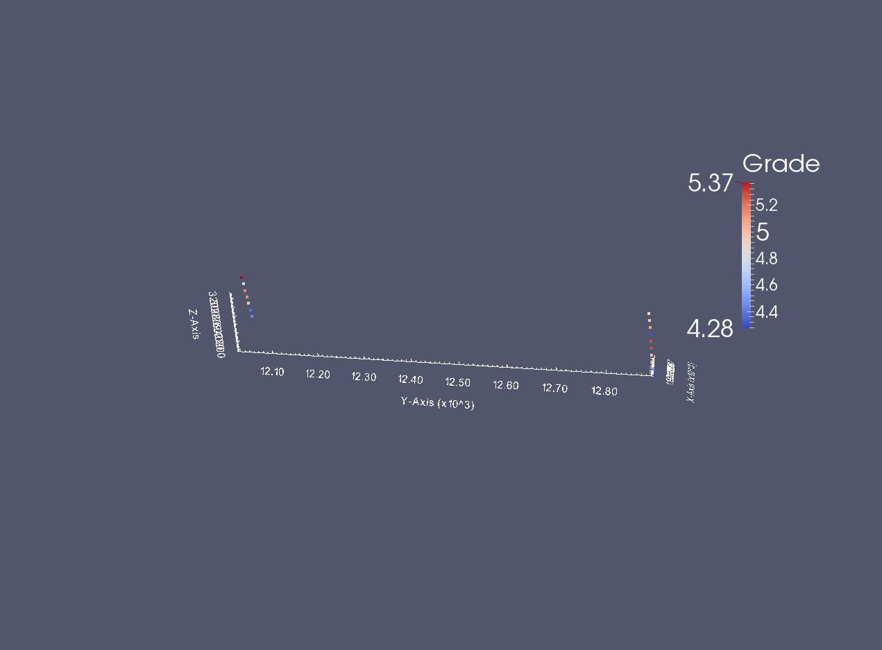
A small screen capture of the desurveyed data

from IPython.display import Image
desurveyedvtk = Image(filename='desurveyed_data_vtk.png')
desurveyedvtk

Writing out a subset of data values¶

Write out just a subset of the data such as grades for a specific category.

print('\nThe bitumen and fines content for fines greater than 40 (first few rows)')
small_dataset = datafl.data[['Bitumen','Fines']][datafl.data['Fines'] > 40.0]
print(small_dataset.head())
datafl.writefile(flname='bit_and_fines_gr_40.dat',fltype='GSLIB',data=small_dataset)

The bitumen and fines content for fines greater than 40 (first few rows)
    Bitumen   Fines
  2.900  43.500
  2.465  44.838
  0.000  52.900
  0.000  52.900
  0.000  52.900

Summary¶

This documentation has demonstrated some of the capabilities of Python + pygeostat. As with all of the tasks we do - there are many ways to accomplish the same thing. Advantages to using Python are that it is a powerful, high level language with hundreds of packages for everything from machine learning algorithms to plotting and a very large userbase which means answers to any question about the language only a google-away. Everything presented here is also 100% free and open source, unlike many other tools such as Matlab and commercial software. There are other advantages for us: Python can dynamically link with C and Fortran code, manage parallel processes across many computers, send you an email when your script is completed… The primary disadvantage is that it is not widely used within CCG so there is limited support and CCG-specific reference material available. This is a significant disadvantage. The depth of reference material and example scripts which are available for Bash and Matlab within CCG is substantial. Python provides just one more alternative!